Confidence intervals (Part 1)
in statistics
January 23, 2022
Introduction
Welcome to another post in my statistics series!
In this post we are going to focus on confidence intervals and try to understand what is their purpose, how to construct them and how to interpret them.
Definition
In a previous post we talked about estimators, desirable properties and how they can be used to estimate quantities of interest. For example, we might have data from a normal distribution and we would like to create an estimator for the mean of that normal.
But this is usually not enough. Being able to say that my estimate for the mean of the normal is 2 will not suffice. More often than not the degree of certainty for that estimate is needed. Can we provide a possible range of values for the unknown quantity with some degree of certainty?
This is where the confidence interval comes into play.
A 1-α confidence interval for a parameter θ is an interval Cn = (A, B) where A = A(X1,…,Xn) and B = B(X1,…,Xn) are functions of the data such that $$ P_{\theta}(\theta ∈ Cn) ≥ 1 − α , \forall θ ∈ Θ$$ In words, (A, B) traps θ with probability 1 − α.
Let’s try to dig deeper into some of the components of the definition.
Cn = (A, B) where A = A(X1,…,Xn) and B = B(X1,…,Xn)
We define the interval in terms of A and B, which are both functions of the samples (X1,…,Xn) we take from the unknown distribution.
1-α confidence interval
It is important to note that we can construct many confidence intervals. The degree of certainty that the interval has is quantified through the number 1-α. For example, if I am 5% certain in my estimate, weeeeell this is probably not a very useful estimate 😅.
Some of the usual values that α takes are 5% (confidence interval 1-α=95%) or 2.5% (confidence interval 1-α=97.5%). Most of the time when constructing an interval we solve for equality (=1-α) in order to find the tightest interval that achieves 1-α confidence.
How does one construct a confidence interval?
We have established so far that in order to construct a confidence interval we need to decide on the level of confidence (1-α) and then calculate the upper and lower limits based on some function of the samples of the unknown distribution. But which function(s) should one take? Let’s have a look through an example.
Uniform distribution [θ-1/2,θ+1/2]
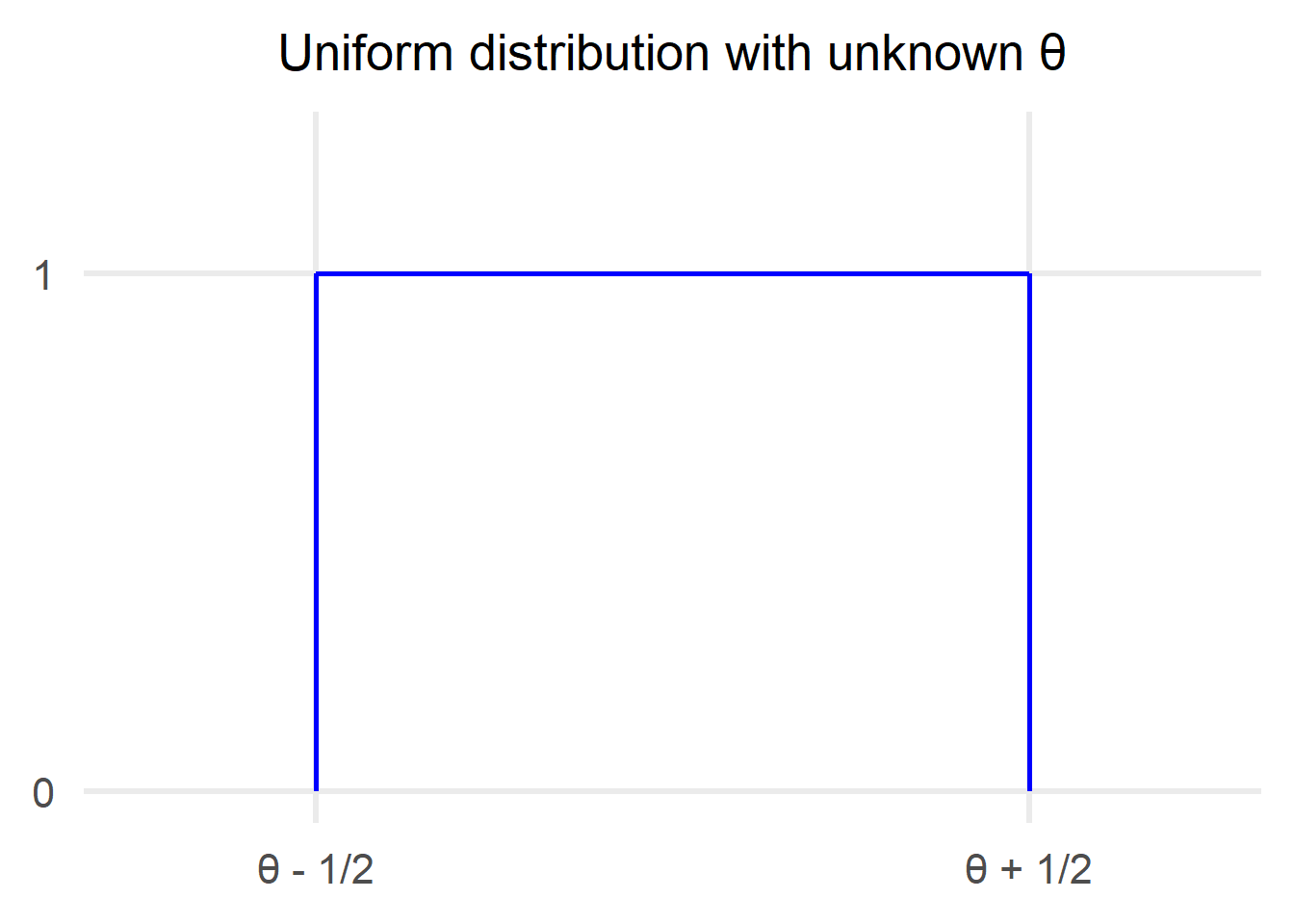
We have the following scenario, a uniform distribution with an unknown parameter θ. We can obtain a number of samples from the distribution: $$X_1, X_2, …, X_n \thicksim U[\theta-1/2,\theta+1/2]\ i.i.d. $$ Furthermore, since this is a uniform we know: $$ E[X] = E[X_1] = … = E[X_n] = \frac {(\theta-1/2+\theta+1/2)} 2 = \theta $$ $$ Var(X)=Var(X_1)=…=Var(X_n) = \frac {(\theta+1/2-(\theta-1/2))^2} {12} = \frac {1} {12} $$ In this scenario the unknown around which we would like to create a confidence interval is the value θ which is the midpoint of the uniform. Therefore, we are trying to find A, B such that:
$$ P_{\theta}(B \ge \theta \ge A) = 1-\alpha , \forall θ ∈ Θ$$
It needs to be stressed again that A and B are functions of the samples obtained from the original unknown distribution, which is why we can make probabilistic statements like the one above.
Step 1: Find a (good!) estimator for θ
The first step for creating a confidence interval is to generate an estimate for the quantity we are interested in. We need to find a good estimator for θ (see my previous post about estimators for more details).
Since E[X] = θ and we know that the sample mean is a good estimator for the expectation we can select it. The sample mean is an unbiased estimator and it is also consistent based on the Law of Large Numbers.
$$ \widehat{\theta}=\overline{X_n} $$
Step 2: Understand the distribution of the estimator (either directly or asymptotically)
Can we say something about the distribution of the sample mean? Yes!
Based on the
Central Limit Theorem as the sample size grows larger the normalised sample mean follows a standard normal distribution asymptotically.
So now we have an estimator (the sample mean) for the unknown quantity θ and we would like to construct an interval using that estimator which will be the asymptotic confidence interval we are looking for. Coming back to our previous definition:
$$ C_n = (A, B) = [\widehat{\theta}-d, \widehat{\theta}+d]=[\overline{X_n}-d, \overline{X_n}+d] $$
Step 3: Calculate the interval limits based on the distribution of the estimator
Based on the definition of the confidence interval and the results of step 1 we want to find d such that:
$$ P_{\theta}(\overline{X_n}+d \ge \theta \ge \overline{X_n}-d) = 1-\alpha , \forall θ ∈ Θ $$ To be more precise, given that we are working with an asymptotic confidence interval, we are looking for an interval that fullfills the condition above as n grows larger:
$$ \lim_{n \rarr \infty}P_{\theta}(\overline{X_n}+d \ge \theta \ge \overline{X_n}-d) = 1-\alpha , \forall θ ∈ Θ $$ In order to find d, we need to make use of the CLT and in particular we need to rearrange the inequality inside the probability to create the normalized version of the sample mean:
$$ P_{\theta}(\overline{X_n}+d \ge \theta \ge \overline{X_n}-d) = P_{\theta}(d \ge \theta-\overline{X_n} \ge -d)=P_{\theta}(d \ge \overline{X_n}-\theta \ge -d) = $$
$$P_{\theta}(\frac {\sqrt{n}d} {\sqrt{1/12}}\ge \sqrt{n} \frac {\overline{X_n}-\theta} {\sqrt{1/12}} \ge \frac {-\sqrt{n}d} {\sqrt{1/12}})$$
Just as a reminder from the CLT we know: $$ \sqrt{n} \frac {\overline{X_n}-\mu} {\sigma} \xrightarrow[n\rarr \infty]{(d)} N(0,1) $$
and this is exactly what we constructed above. We subtracted the expectation (θ) from the sample mean, divided by the square root of the variance and multiplied by square root n.
Now we can substitute the middle part $$ \sqrt{n} \frac {\overline{X_n}-\theta} {\sqrt{1/12}} $$ with the standard normal distribution Ζ:
$$ P(\frac {\sqrt{n}d} {\sqrt{1/12}}\ge Z \ge \frac {-\sqrt{n}d} {\sqrt{1/12}}) $$
We would like this probability to be equal to 1-α.
$$ P(\frac {\sqrt{n}d} {\sqrt{1/12}}\ge Z \ge \frac {-\sqrt{n}d} {\sqrt{1/12}}) = 1-α $$ To simplify calculations, we set $$ \frac {\sqrt{n}d} {\sqrt{1/12}} = e $$ and we have (have a look at my previous post about the normal distribution in case these calculations here seem fuzzy): $$ P(e \ge Z \ge -e) = 1-α \hArr \Phi(e) - \Phi(-e)=1-α \hArr 2\Phi(e)-1=1-α \hArr$$ $$ \Phi(e)=1-\frac α 2 \hArr e=\Phi^{-1}(1-\frac α 2)=q_{\alpha/2}$$
By solving this equation we establish that e has to be equal to the a/2 quantile of the normal distribution. Let’s put this value back in the original equation to calculate the value of d:
$$ \frac {\sqrt{n}d} {\sqrt{1/12}} = q_{\alpha/2}\hArr d= \frac {q_{\alpha/2}} {\sqrt{12n}}$$
The only thing we have left is to put all the ingredients together:
Our estimate for θ is: $$ \overline{X_n} $$ The 1-α asymptotic confidence interval for θ is: $$ C_n = (A, B) = [\overline{X_n}-\frac {q_{\alpha/2}} {\sqrt{12n}}, \overline{X_n}+\frac {q_{\alpha/2}} {\sqrt{12n}}] $$
In action
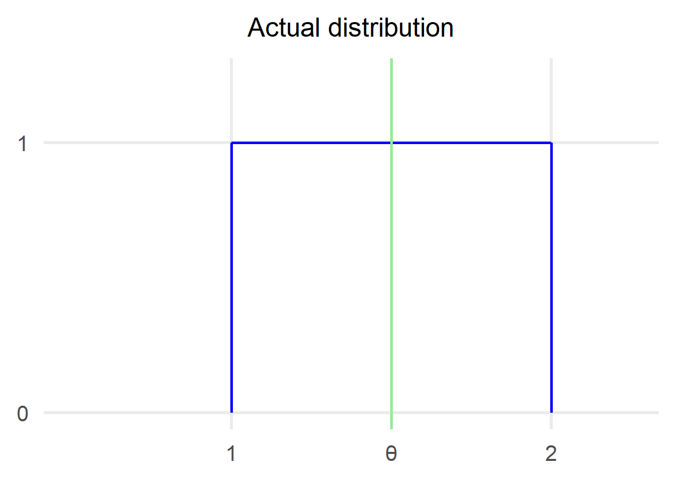
But enough theory, let’s try it out in practice. The actual distribution we are going to use is a U[1,2] and we are going to calculate a 95% confidence interval:
We are going to first draw 50 samples from the distribution:
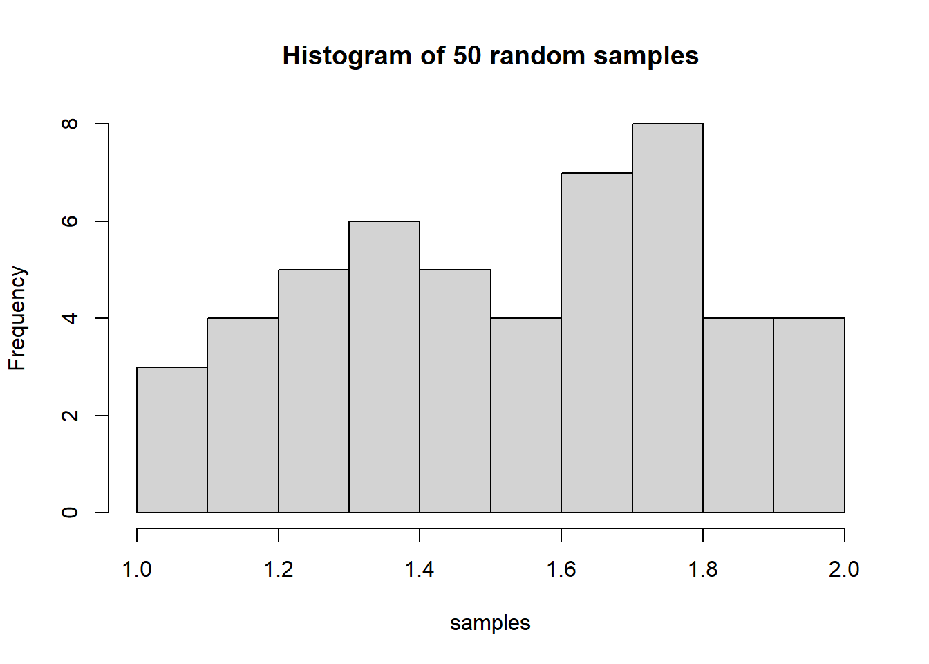
Let’s calculate all the quantities we derived in the theoretical calculations:
The sample mean is equal to 1.53
N is equal to 50
The 0.025 quantile of the standard normal is 1.96
The interval lower limit is 1.45
The interval upper limit is 1.61
Putting these values back into the formula we derived above, we can say that a 95% asymptotic confidence interval for the unknown parameter θ is:
$$ [1.45, 1.61] $$
Note that we cannot make probabilistic statements about these numbers, which means we cannot say: $$ \cancel{P(1.61 \ge \theta \ge 1.45) = 1-\alpha , \forall θ ∈ Θ}$$
The reason is that once we have a realisation (numbers) for the confidence interval, the probability that the unknown θ is in the realised confidence interval is either 0 (θ is not in that interval) or 1 (θ is in that interval). θ is unknown but it is not random!
Interpreting the confidence interval
It is crucial to understand how to interpret a confidence interval. A 95% confidence interval tells us that if we rerun the same experiment 100 times the true value of the quantity we are trying to estimate (in our example it was θ) will be included in 95 out of the 100 intervals. Luckily for us we can rerun the above calculations 100 times in R and see whether the statement is true:
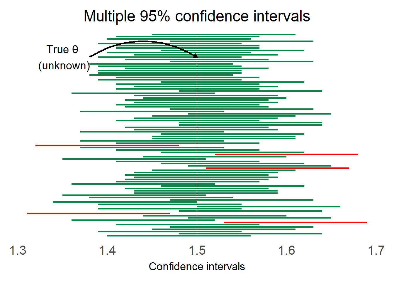
The intervals marked in green contain the true value of θ which in this example is 1.5. There are 5/100 intervals that do not contain the value and I have marked them in red. Please note that the value of 5 does match our expectation that 95 of the intervals would contain the true value but this is not always the case, it could have been 4 or 6 or some other number close to that.
Useful resources
Wikipedia
All of statistics book
Fundamentals of statistics course at edX
- Posted on:
- January 23, 2022
- Length:
- 8 minute read, 1499 words
- Categories:
- statistics
- Tags:
- statistics