The Central Limit Theorem
in statistics
December 11, 2021
Introduction
This is my second post in the Statistics series. ( Previous post about the Law of Large Numbers) The aim of this series is to present various statistical topics in an easy to grasp visual way without going very deep in mathematical formulas.
The topic of this post is the Central Limit Theorem.
Definition
The Central Limit Theorem establishes that, in many situations, when independent random variables are summed up, their properly normalized sum tends toward a normal distribution (informally a bell curve) even if the original variables themselves are not normally distributed.
Let’s try to map the words in the definition to mathematical constructions.
Independent random variables
Here we assume that we have n random variables with the same underlying probability distribution.
These random variables are independent and identically distributed (i.i.d.).
Furthermore, they have the following characteristics:
Properly normalized sum
Normalising the sum of these variables means creating a new random variable with an expected value of 0 and variance of 1. Let’s see how this can be done in practice.
We start out with the sum of the random variables we defined above and we will also give it a name so that we can work with it more easily.
The expectation of A is:
(1) is possible via the linearity of expectations.
The variance of A is:
Linearity unfortunately does not hold for the variance. So under normal circumstances:
But this is where our assumption of independent random variables comes into play to save the day. Linearity holds in the case of independence as the covariances between the variables are all equal to 0. Which means:
Now we know the expected value and the variance of the random variable A. What we need to do is to make some manipulations to construct a new random variable from it with expected value equal to 0 and variance equal to 1.
Expected value equal to 0
This is the easier of the two as we simply need to subtract the expected value of A from A. Let’s see that:
(1) The expectation of a constant (nμ) is equal to the constant
Variance equal to 1
In order to set the variance to 1 we need to divide the random variable by the square root of its variance:
(1) The variance of a constant (nμ) is 0
(2) Properties of variance:
Putting both results together we can create the properly normalized sum:
Tends toward a normal distribution
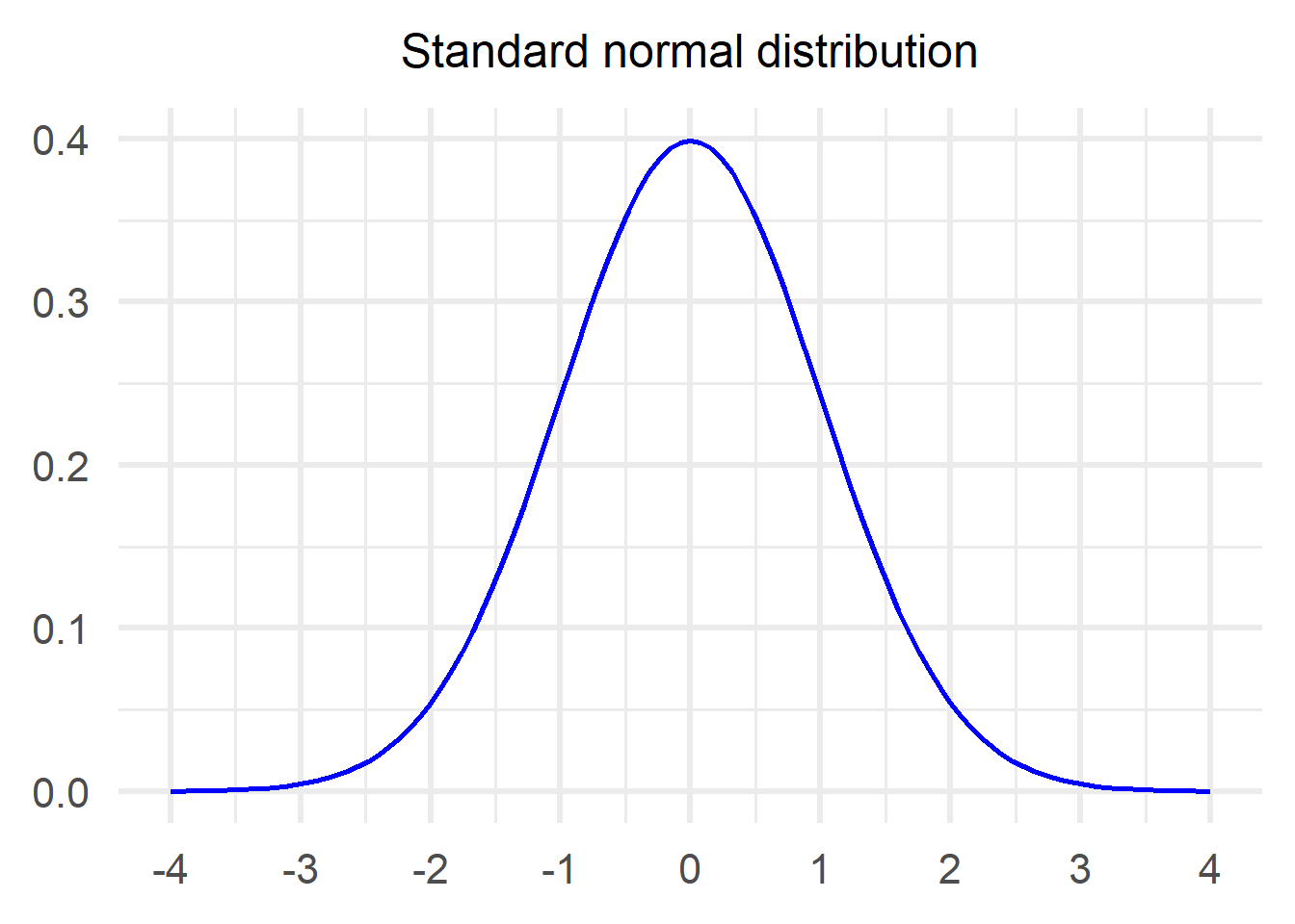
This is the most crucial part of the theorem and what it states is that the distribution of the properly normalized sum we created above will be very similar to a standard normal distribution. Just as a reminder, this is what a standard normal distribution looks like:
In mathematical notation the Central Limit Theorem looks like this:
Let’s take a minute to digest what the theorem says:
Without making any assumptions about the distribution of the initial random variables (Xi), it tells us that if you take many of them (n), sum and normalize them, their normalized sum will follow approximately a standard normal distribution.
This is an incredible statement to make with so little knowledge!
Equivalent formulations
Depending on the book/course/class, there are equivalent formulations of the CLT that might be used (I was very confused by those initially). Here are some of them and what manipulation is used:
The following formulation is the one I will use for the rest of the post (and I think it is the most popular one) Dividing both the numerator and the denominator by n to create the sample mean
Multiplying both sides by σ to remove the denominator
Moving everything to the right side by dividing by √n and adding μ
Population, sample and number of experiments
As you can imagine, in order to see whether the theorem holds and how it looks like in practice we need to compare the actual normalized sample mean distribution with the normal distribution (which is the theoretical one we approach in the limit).
Based on the formula above, all we need is the Xi, μ, σ and n.
But here take pause. Imagine that I give you n=30, specify the realisations of all 30 Xis as well as μ and σ. Put them all together and what you have is a single value. How are we supposed to compare that with a distribution?
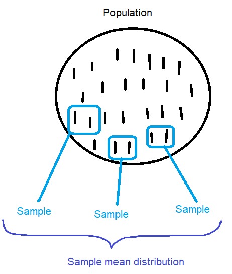
In order to understand the process better let’s define the concepts of population, sample and number of experiments through an example: Voting
Imagine there are elections in the country and we would like to estimate the outcome through polling.
The most reliable way to do this is to ask everyone in the country what they voted. The total population of the country is the population of the experiment.
But as you can imagine, it is not always easy to get your hands on the population. For various reasons (money, time, etc.) we might be able to poll only a subset of the population in order to produce an estimate. For example it could be that we can only poll 50 people. This is a sample with a sample size of 50.
Lastly, in a theorem such as the CLT we are talking about the distribution of the normalised sample mean. Every normalised sample mean (with a sample size n large enough) follows the normal distribution but we can only see a representative picture of that distribution if we repeat the process multiple times. Therefore, we need increase the number of experiments that we run.
Pictorially it looks like this:
⚠️ The naming convention that I used in the paragraph above is how I understand the process. Unfortunately, I could not find consistent naming conventions. If you have any suggestion that is clearer/more widely accepted, please let me know!
In action
1. Uniform distribution
In our first example, we assume the following:
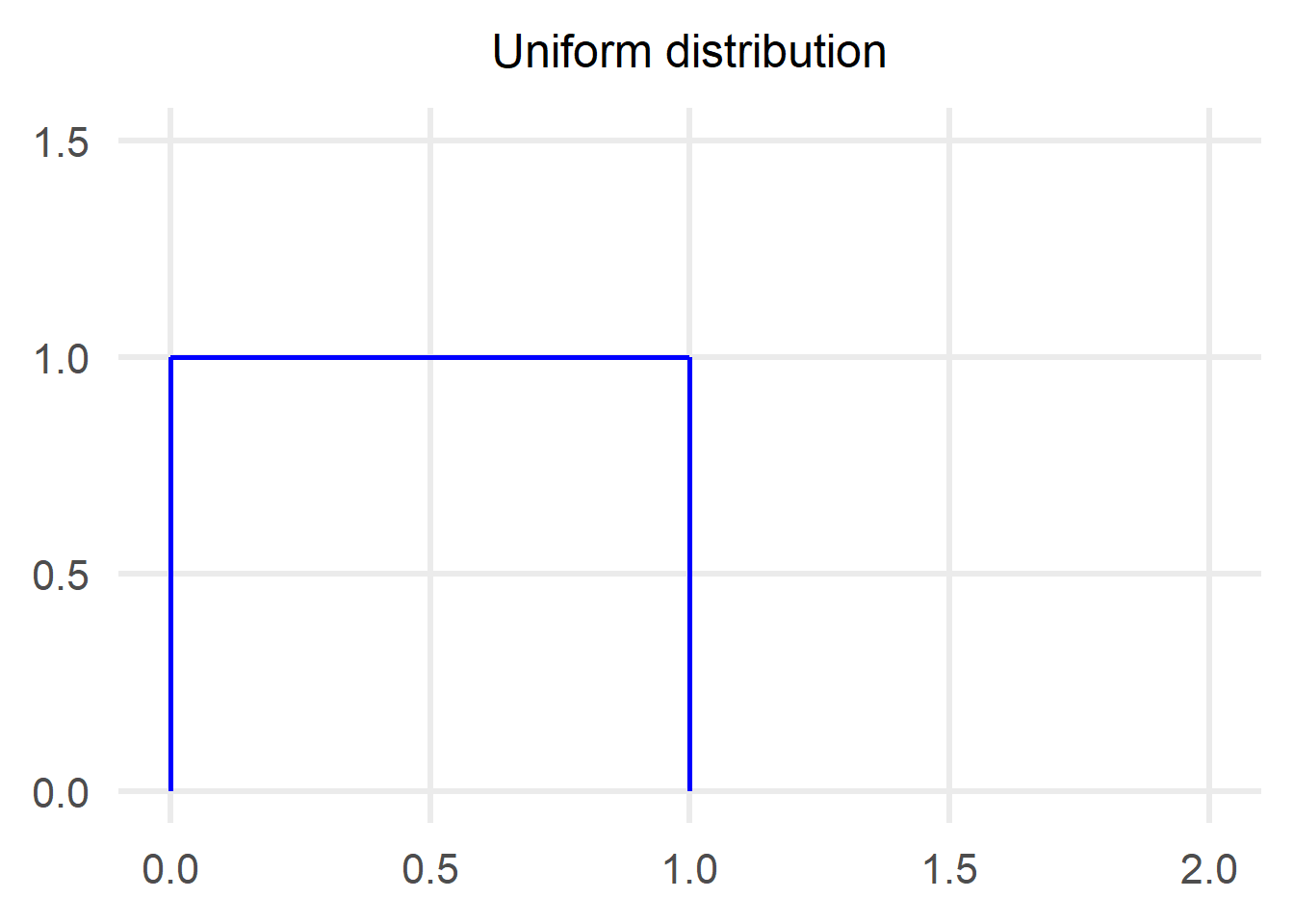
We need the expected value and the variance of the distribution to proceed:
Therefore we have:
The process we are going to follow in order to compare with the normal distribution is the following:
- Pick a sample size
- Perform multiple experiments using the determined sample size and keep track of the sample mean for each experiment
- Normalise the sample means
- Convert the results into a histogram and compare with the normal distribution
Let’s see how steps 1-3 look like.
Performing 100 experiments with a sample size of 50
The next step is to convert the above dot plot into a histogram:
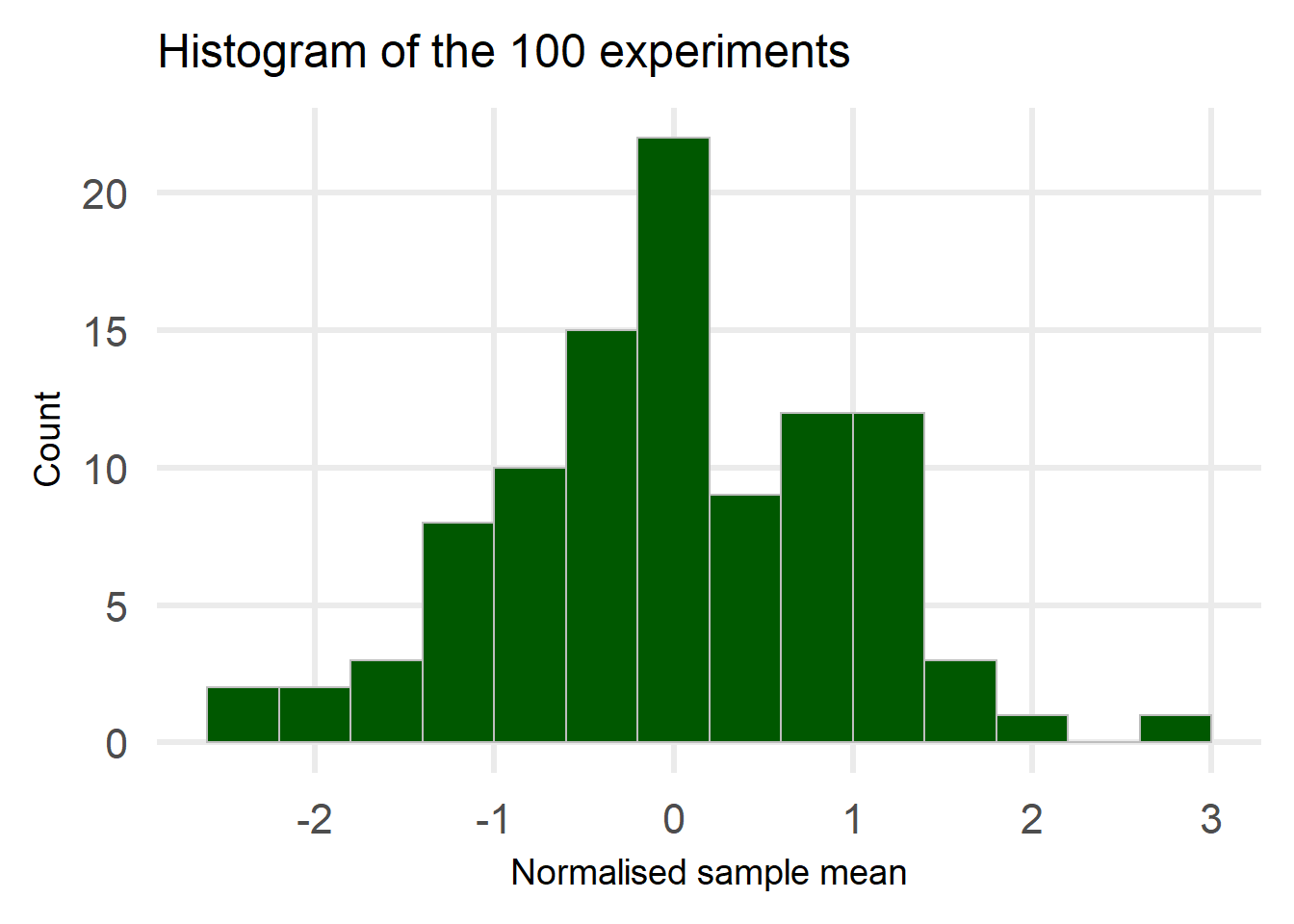
The histogram is nothing more than the points from the previous plot converted into bars.
One problem remains before we do the comparison: The histogram currently counts the number of experiments that fell into each bin but we want to compare this to a normal distribution.
The solution to this problem is to switch from count to frequency, e.g. if a bin contains 10 experiments and we have performed 100 experiments in total then the frequency of that bin is 10/100=0.1.
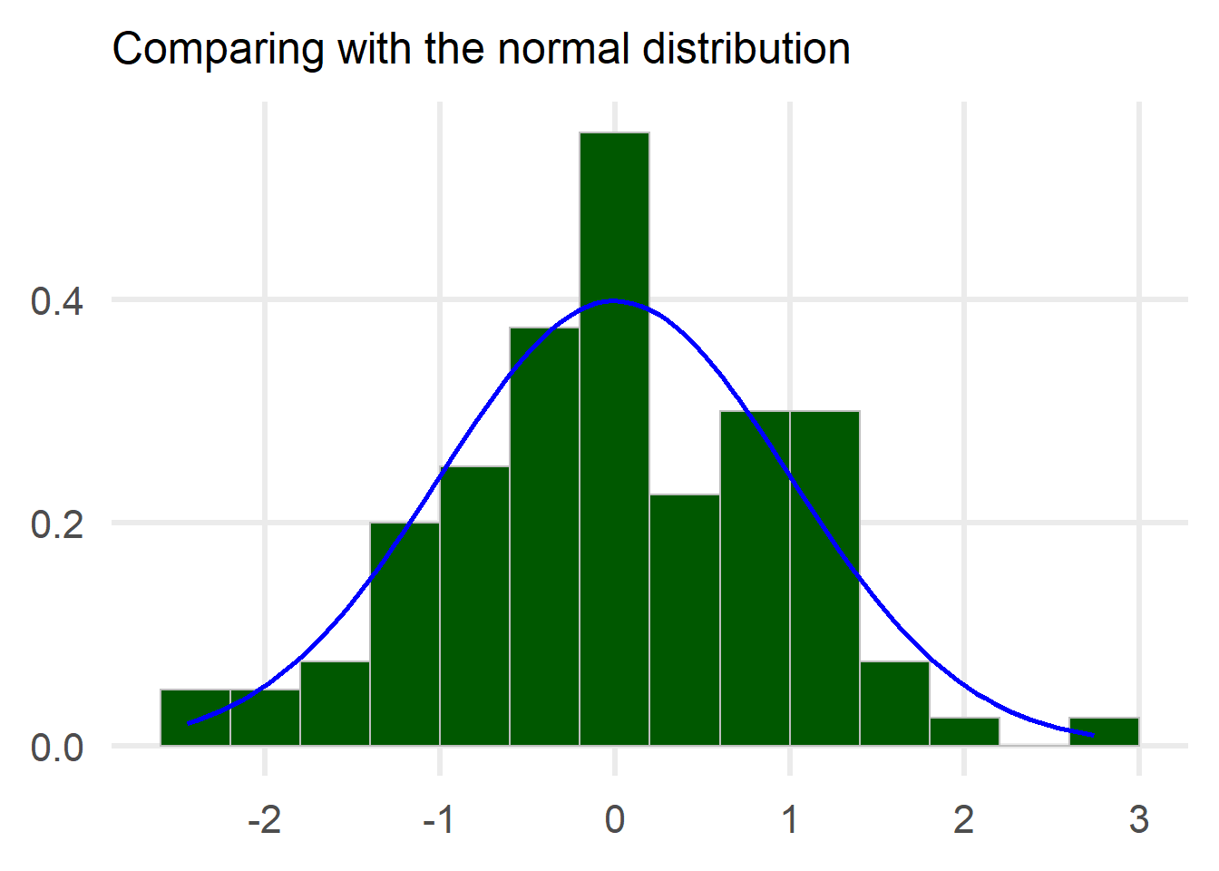
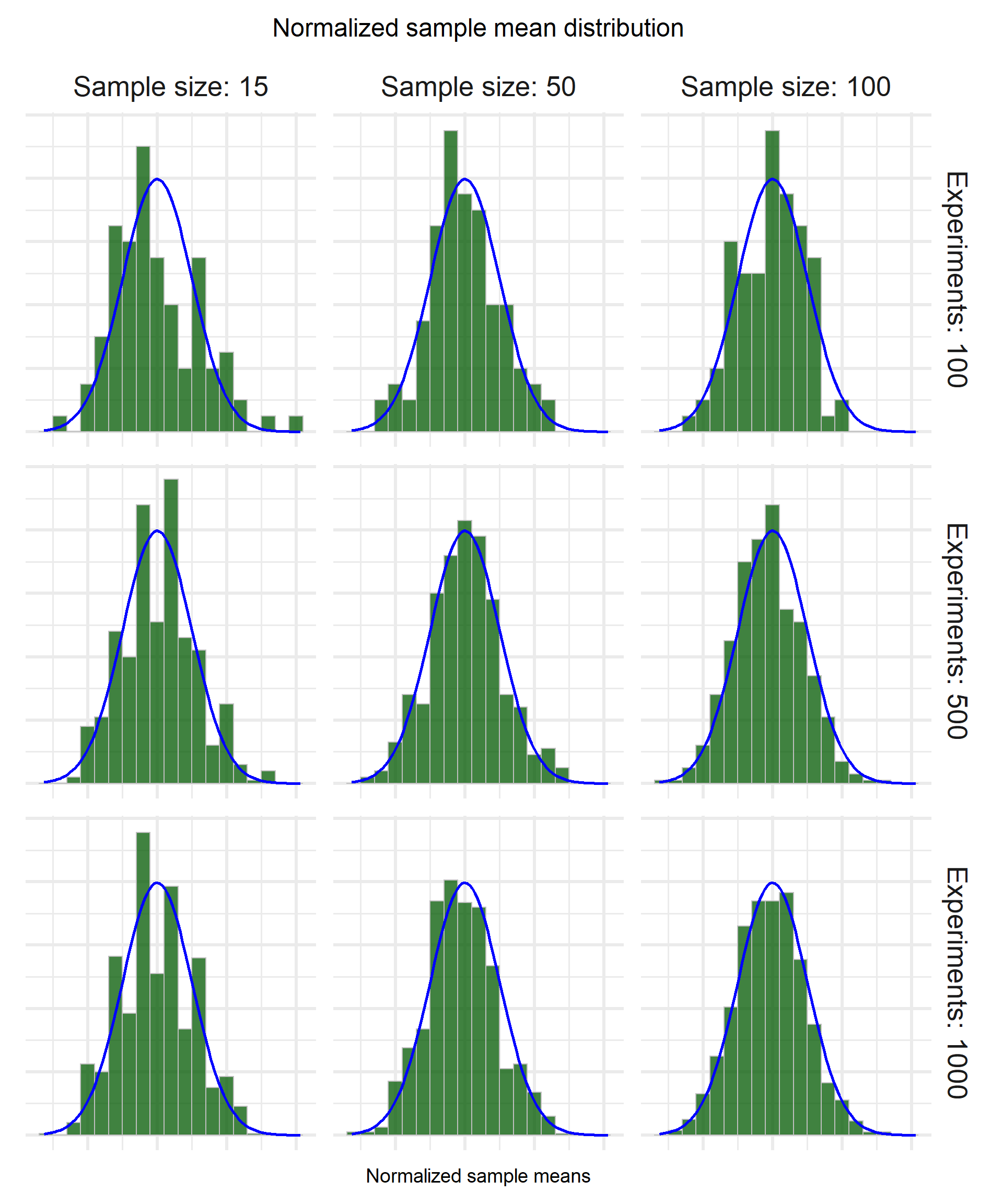
Hooray!! We managed to establish a procedure with which we can compare to a normal distribution!! Let’s see now how the comparison looks like for various sample sizes / number of experiments.
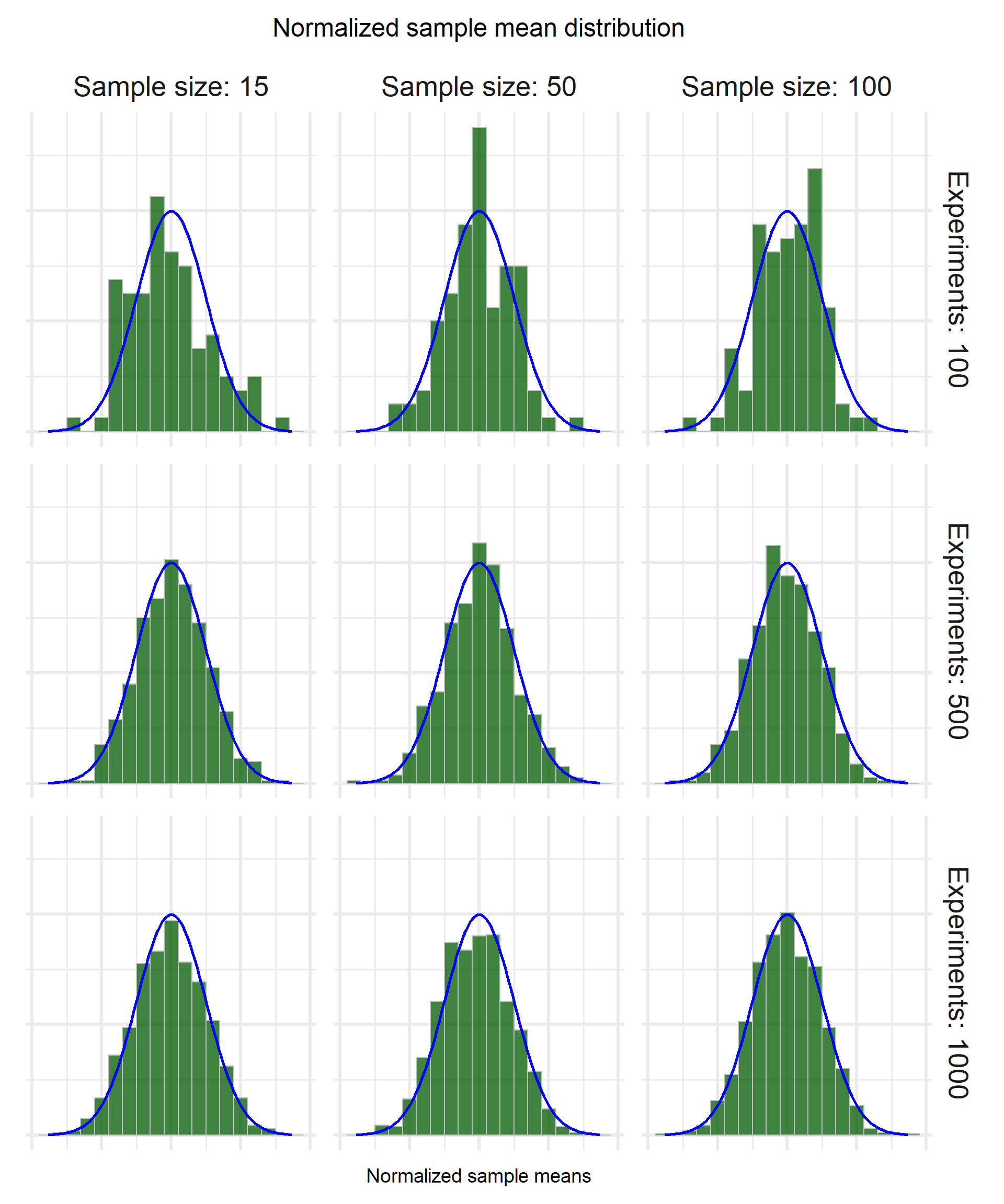
We can clearly see that the number of experiments is the determining factor in how the distribution looks like. For example, in the first row where we have 100 experiments, the distribution does not fit the ideal normal so snugly regardless of how big the sample size is.
Once we increase the number of experiments to 500 or 1000, even for small sample size (15) the distribution is a tight fit.
2. Poisson distribution
The second distribution we are going to use for exploring the Central Limit Theorem is the Poisson, with a value of λ=1.
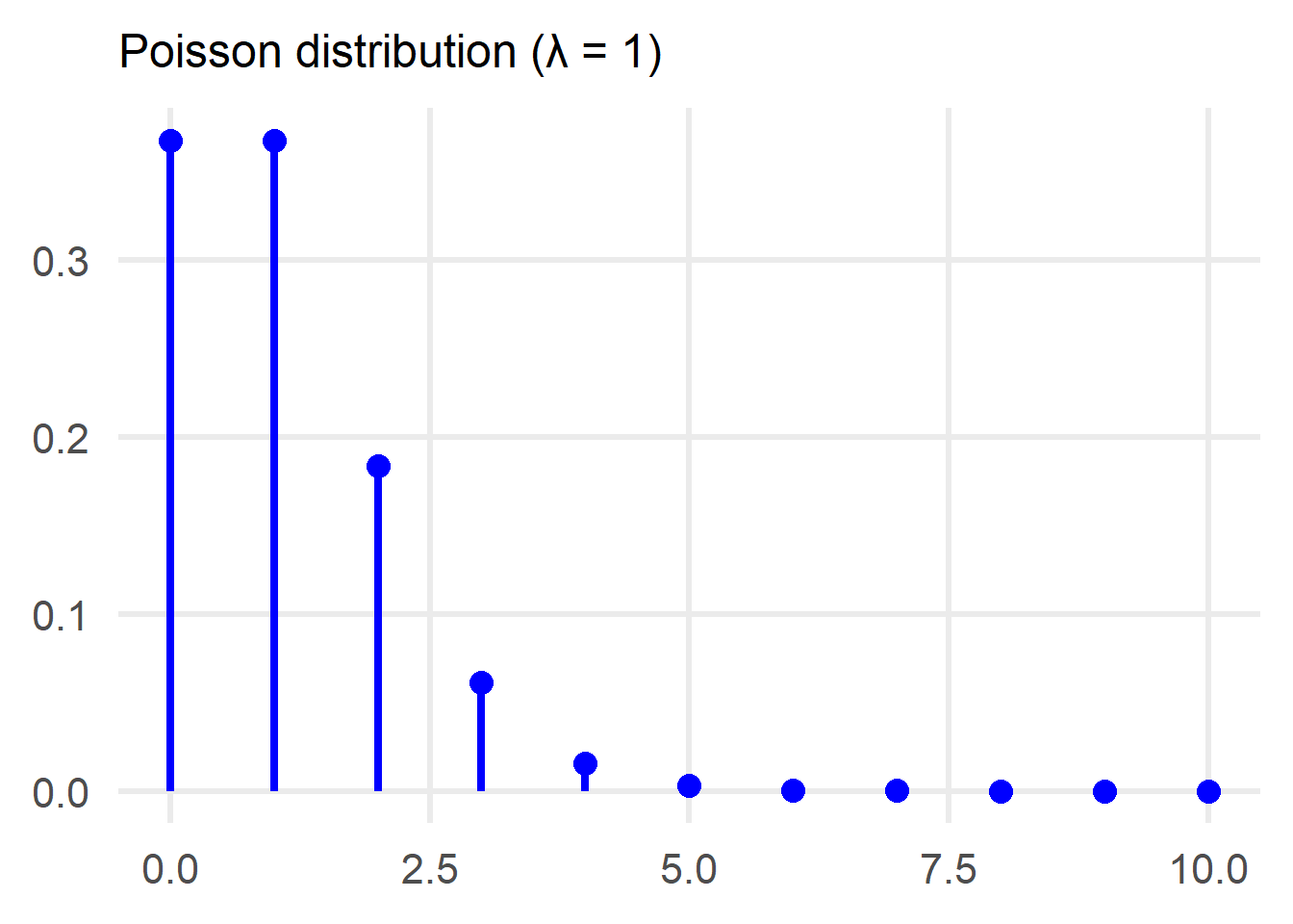
Once again we need the expected value and the variance of the distribution to proceed:
Therefore we have:
The process we follow is exactly the same as before, so I am going to skip straight to how the results look like by sample size/number of experiments.
The results are very interesting! For sample size 15 the distribution of the normalized sample mean looks kinda normal but far from the ideal regardless of the number of experiments. Once we increase the sample size, we reach the ideal shape especially for a larger number of experiments.
Why is this cool?
The Central Limit Theorem allows us with very little prior knowledge of a distribution (mean and variance) to say things about the distribution of its sample mean. This is a very powerful result that we can leverage when trying to make estimates for the unknown distribution.
Or
as Josh Starmer says: “Even if you’re not normal, the average is normal!!
- Posted on:
- December 11, 2021
- Length:
- 8 minute read, 1681 words
- Categories:
- statistics
- Tags:
- statistics